Is co-Kriging always better than ordinary Kriging?
A new discussion on the performance of co-Kriging and ordinary Kriging.
1. Common discussions on CK and OK
There have been many discussions about the comparison between co-Kriging (CK) and
ordinary Kriging (OK) in terms of prediction error and variance. For example, a
technical note
about CK with gstat package in R compares CK and OK using different co-variates with different strength of correlation with the response.
Also, the documentation of CK in ArcGIS
mentions that “theoretically, you can do no worse than kriging because if there is no cross-correlation,
you can fall back on autocorrelation for the response.”
To summarize, a common conclusion is that
- if there is a strong correlation between a covariate and the response, CK would make better prediction than OK, otherwise, CK would make no better prediction than OK.
So, the answer to the question is “no”, as CK is better than OK only if there exist strong correlations between covariates and response. The “better” means smaller prediction error and variance.
2. A new discussion
The conclusion above is not strictly accurate or reliable for all situations, as in many conditions, even with strong correlated covariates, the outperformance of CK compared to OK is still hard to notice. So, a new problem would be
- when and why doesn’t CK outperform OK?
Previous discussions focus on testing the influence of the correlation strength between covariates and response. However, considering that Kriging is to make predictions at unknown locations based on known sampling locations and a previous post mentions that CK is used when auxiliary variables are available but not available at all grid-nodes, therefore,
- the sampling size and locations should affect the performance of CK a lot in real practice.
A paper titled “When Doesn’t Cokriging Outperform Kriging” discussed the problem theoretically. The conclusions are
- CK is identical to OK when the sampling locations of auxiliary variables is the same with or is a subset of locations where the response variable is observed.
- CK might outperform OK when the auxiliary variable is observed at more locations than the response variable.
The above conclusions are quite intuitive and not hard to understand. A case study using gstat package with the commonly used “meuse” data in R is conducted to validate the above conclusions.
(0). Select strongly correlated zinc (zn) and lead (pb) as response and covariate, respectively.
library(sp)
library(gstat)
library(ggplot2)
library(lattice)
library(gridExtra)
#================
# 0. load data
#================
data(meuse)
data(meuse.grid)
# 0.1 test strength of corrleation
xyplot(log10(meuse$lead)~log10(meuse$zinc))
cor(log10(meuse$lead), log10(meuse$zinc))
# 0.2 log transformation of lead and zinc data
meuse <- cbind(meuse, logpb = log10(meuse$lead), logzn = log10(meuse$zinc))
(1). Sample training and test data. Make sure zinc and lead are sampled at the same locations in the training data. Conduct OK and CK respectively and calculate their prediction RMSE for test data. The RMSE for OK and CK are RMSE.OK = 0.166, RMSE.CK1 = 0.182, which demonstrate CK does not outperform OK when the sampling of covariate is the same with the sampling of response.
#======================================================================
# 1. response zinc and covariate lead are sampled at the same locations
#======================================================================
# 1.1 sample training and test data
meuse.train <- meuse[seq(1, length(meuse$logzn), by=3),
                     c("x", "y", "logpb", "logzn")]
meuse.test <- meuse[setdiff(rownames(meuse), rownames(meuse.train)),
                    c("x", "y", "logpb", "logzn")]
coordinates(meuse.train) = ~ x+y
coordinates(meuse.test) = ~ x+y
# 1.2 ordinary kriging for zinc
# fit variogram
ok.vgm <- variogram(logzn~1, meuse.train)
ok.fit <- fit.variogram(ok.vgm, model = vgm(0.08,"Exp",800,0.03))
plot(ok.vgm, ok.fit)
# krige predict based on variogram
ok.kriged <- krige(logzn~1, meuse.train, meuse.test, model = ok.fit)
RMSE.OK <- sqrt(sum((meuse.test$logzn-ok.kriged$var1.pred)^2)/dim(meuse.test)[1])
# 1.3 co-Kriging for zinc
ck.g <- gstat(id = "logzn", formula = logzn ~ 1, data = meuse.train)
ck.g <- gstat(ck.g, id = "logpb", formula = logpb ~ 1, data = meuse.train)
ck.g <- gstat(ck.g, model = vgm(0.08,"Exp",800,0.03), fill.all=T)
ck.vario <- variogram(ck.g)
ck.vario.fit <- fit.lmc(ck.vario, ck.g, fit.method = 1)
plot(ck.vario, ck.vario.fit)
ck.pred <- predict(ck.vario.fit, newdata = meuse.test)
RMSE.CK1 <- sqrt(sum((meuse.test$logzn-ck.pred$logzn.pred)^2)/dim(meuse.test)[1])
(2). Conduct another sampling for lead and make it have more samples than zinc. The prediction RMSE is RMSE.CK2 = 0.087 which is much smaller than the previous OK and CK prediction. Therefore, for this case, CK outperforms OK when the covariate is sampled with more density than the response.
#======================================================================
# 2. covariate lead are sampled to have more samples than response zinc
#======================================================================
meuse.train_zn <- meuse[seq(1, length(meuse$logzn), by=3),
                     c("x", "y", "logzn")]

meuse.train_pb <- meuse[, c("x", "y", "logpb")]

meuse.test <- meuse[setdiff(rownames(meuse), rownames(meuse.train_zn)),
                      c("x", "y", "logpb", "logzn")]
coordinates(meuse.train_zn) = ~ x+y
coordinates(meuse.train_pb) = ~ x+y
coordinates(meuse.test) = ~ x+y
# 2.1 co-Kriging for zinc
ck.g2 <- gstat(NULL, id = "logzn", formula = logzn ~ 1, data = meuse.train_zn)
ck.g2 <- gstat(ck.g2, id = "logpb", formula = logpb ~ 1, data = meuse.train_pb)
ck.g2 <- gstat(ck.g2, model=vgm(0.08,"Exp",800,0.03), fill.all=T)
ck.vario2 <- variogram(ck.g2)
ck.vario2.fit <- fit.lmc(ck.vario2, ck.g2, fit.method = 1)
plot(ck.vario2, ck.vario2.fit)
ck.pred2 <- predict(ck.vario2.fit, newdata = meuse.test)
RMSE.CK2 <- sqrt(sum((meuse.test$logzn-ck.pred2$logzn.pred)^2)/dim(meuse.test)[1])
(3). To visualize the difference, predictions are made on “meuse.grid” data using OK, CK1, and CK2 respectively.
#==========================
# 3. predict on meuse.grid
#==========================
coordinates(meuse.grid) = ~ x+y
OK.grid <- krige(logzn~1, meuse.train, meuse.grid, model = ok.fit)
CK1.grid <- predict(ck.vario.fit, newdata = meuse.grid)
CK2.grid <- predict(ck.vario2.fit, newdata = meuse.grid)
# show results
df<- data.frame(meuse.grid, OK = OK.grid$var1.pred, CK1 = CK1.grid$logzn.pred,
                CK2 = CK2.grid$logzn.pred)
p1 <- ggplot(df, aes(x, y)) +
  geom_tile(aes(fill=OK)) +
  scale_fill_gradientn(colours = rainbow(10)) +
  ggtitle("OK prediction") + theme(plot.title = element_text(hjust = 0.5),
                                   axis.text.x=element_blank(),
                                   axis.text.y=element_blank(),
                                   aspect.ratio=1)
p2 <- ggplot(df, aes(x, y)) +
  geom_tile(aes(fill=CK1)) +
  scale_fill_gradientn(colours = rainbow(10)) +
  ggtitle("CK prediction1_|S(zn)|=|S(pb)|") + theme(plot.title = element_text(hjust = 0.5),
                                   axis.text.x=element_blank(),
                                   axis.text.y=element_blank(),
                                   aspect.ratio=1)
p3 <- ggplot(df, aes(x, y)) +
  geom_tile(aes(fill=CK2)) +
  scale_fill_gradientn(colours = rainbow(10)) +
  ggtitle("CK prediction2_|S(zn)|<|S(pb)|") + theme(plot.title = element_text(hjust = 0.5),
                                   axis.text.x=element_blank(),
                                   axis.text.y=element_blank(),
                                   aspect.ratio=1)
grid.arrange(p1, p2, p3, nrow=2, ncol=2)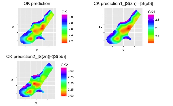
As can be seen from the figure, OK prediction is almost the same as CK prediction1 when the sampling locations of zinc and lead are the same. When more lead data are sampled, CK prediction2 becomes quite different from OK prediction and CK prediction1.