Spatial partition-wise/region-wise/segmented/piecewise regression
Partitioning a 2D space for piecewise regression.
1. Introduction
Piecewise regression is a common technique dealing with non-stationary (varying coefficient) linear model of dependent-independent variables. There have been many methods dealing with input space segmentation for building piecewise regression models, e.g., treed model, dynamic programming for the fixed design segmented regression. However, there is a lack of methods specifically dealing with 2D-spatial partition-wise regression. This post adopts a greedy merging algorithm that efficiently and automatically detects the change-points (boundaries) of the spatially piecewise relationship. The algorithm borrows ideas from a paper ‘Fast Algorithms for Segmented Regression’ and a GitHub repository DataDog/piecewise.
2. Algorithm
-
Input: 2D spatially distributed independent variables at spatial locations , and corresponding dependent variable .
-
Output: a 2D space is partitioned into regions: , which have different regression models.
-
Make an initial segmentation of the 2D space, e.g., partition the space into multiple uniform rectangle grids. Fit a linear model within each region, and calculate the summation of the fitting errors of all regions, e.g., the sum of squared errors, ;
-
Iterate the following two steps until or the number of regions reduced to one:
- For every pair of neighboring regions, calculate the increase of fitting errors () after merging;
- Merge the pair of neighboring regions with the smallest increase of fitting errors.
-
Note that is the number of iterations. is a predetermined threshold, e.g., . is the sum of squared errors and can be replaced with other metrics, such as the sum of absolute errors.
-
The Matlab code of the algorithm and an example can be found in GitHub@jay15summer.
3. An example
To demonstrate the effectiveness of the above algorithm, a simulation case study was made.
- A 2D space was first simulated by:
  [s1, s2] = meshgrid(1:0.1:10,1:0.1:10);
  s1 = reshape(s1, size(s1,1)*size(s1,2),1);
  s2 = reshape(s2, size(s2,1)*size(s2,2),1);
  S = [s1 s2];% locations
- Two independent variables were simulated at locations by:
  X1 = normrnd(2, 0.5, length(S), 1);% independent variable 1
  X2 = normrnd(1, 0.1, length(S), 1);% independent variable 2
  X = [X1 X2];
- Dependent variable was simulated based on a piecewise linear model of -:
  Y = zeros(length(S), 1); % initialize dependent variable
  % simulate partition-wise regression with varying coefficients (varying
  % sharply with crisp boundary)
  for i = 1: length(S)
      if S(i, 1) < 3 && S(i, 2) < 5
          Y(i) = 1 + 2*X1(i) + X2(i) + normrnd(0, 0.2);
      elseif S(i, 1) < 6 && S(i, 2) < 8
          Y(i) = 1.5 + 3*X1(i) + 2*X2(i) + normrnd(0, 0.2);
      else
          Y(i) = 2 + 3.5*X(i) + 1.5*X2(i) + normrnd(0, 0.2);
      end
  end
- Automatic partitioning was implemented based on the proposed algorithm (the code of
spatial_partition_regand its descriptions can be found in GitHub@jay15summer):
  % main function for spatial partitioning
  h = 9; v = 9; T = 0.1;
  [partition_all, partition_slt] = spatial_partition_reg(S, X, Y, h, v, T);
- The partitioning results and the percentage of SSE increase for every merging are as follows:
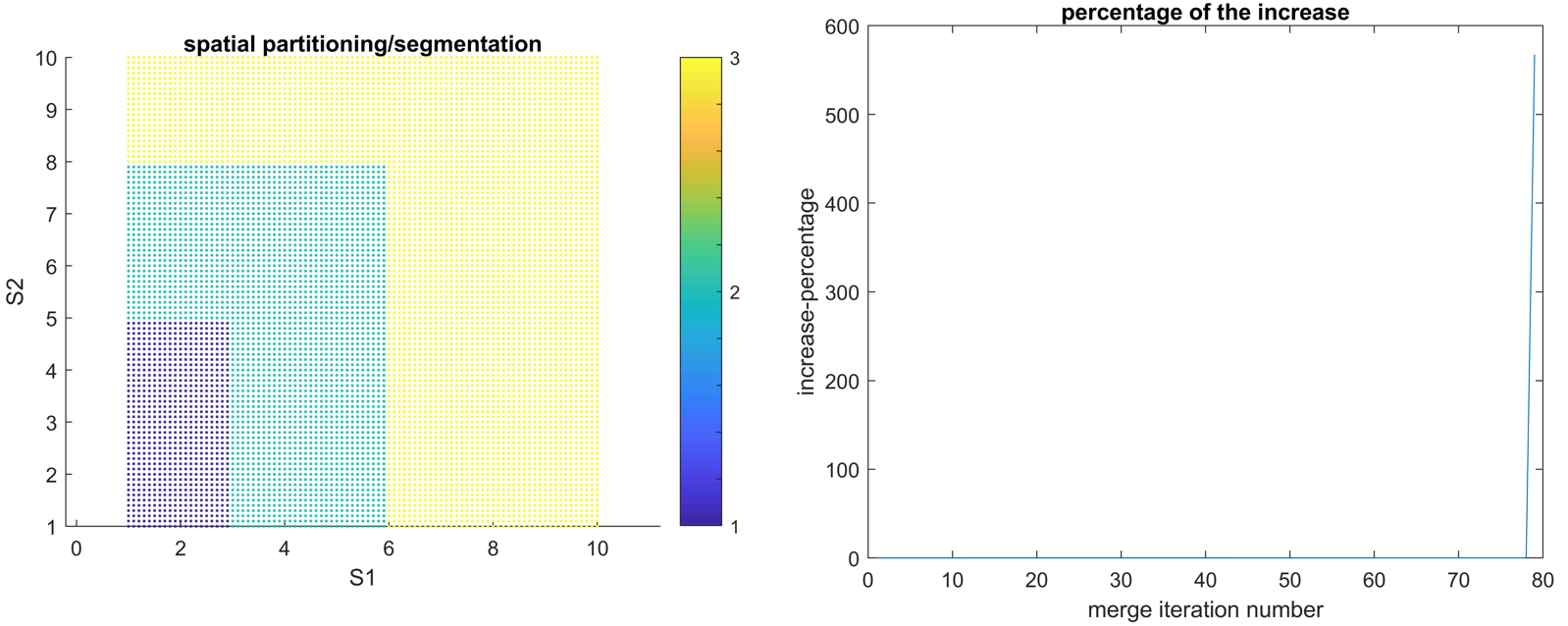 Spatial partitioned regions and the percentage of SSE increase during merging process.
 - It can be seen that the algorithm correctly partitioned the 2D space into three regions as they were simulated.
4. Related problem
In many situations, the change of the relationship of independent-dependent variables has no clear spatial boundaries. Under such conditions, the piecewise assumption is violated, and the algorithm may not result in good partitioning. To deal with such problem, local models can be applied instead, such as geographically weighted regression (GWR) model (refer to http://gwr.maynoothuniversity.ie/ or GWR-in-ArcGIS).